

Cloud Mask Algorithm
The strategy for clear vs. cloudy discrimination in a given MODIS FOV is as follows:
- Perform various spectral and/or spatial variability tests appropriate to the given scene and illumination characteristics to detect cloud presence
- Calculate clear-sky confidences for each test applied
- Combine individual test confidences into a preliminary overall confidence of clear sky for the FOV
- If necessary, apply clear-sky restoral tests appropriate for the given scene type, illumination, and preliminary confidence value
- Determine final output confidence as one of four categories: confident clear, probably clear, probably cloud, or confident cloud
The details of this process follows. Test thresholds have been determined using several methods: 1) from heritage algorithms mentioned above, 2) manual inspection of MODIS imagery, 3) statistics derived from collocated CALIOP (Cloud-Aerosol Lidar with Orthogonal Polarization) cloud products and MODIS radiance data, and 4) statistics compiled from carefully selected and quality controlled MODIS radiance data and MOD35 cloud mask results. The method for combining results of individual cloud tests to determine a final confidence of clear sky is detailed below.
Theoretical Description of Cloud Detection
The theoretical basis of the spectral cloud tests and practical considerations are contained in this section. For nomenclature, we shall denote the satellite measured solar reflectance as R, and refer to the infrared radiance as brightness temperature (equivalent blackbody temperature determined using the Planck function) denoted as BT. Subscripts refer to the wavelength at which the measurement is made.
INFRARED BRIGHTNESS TEMPERATURE THRESHOLDS AND DIFFERENCE (BTD) TESTS
The azimuthally averaged form of the infrared radiative transfer equation is given by
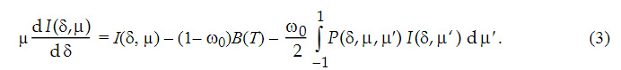
In addition to atmospheric structure, which determines B(T), the parameters describing the transfer of radiation through the atmosphere are the single scattering albedo, ω0 = σsca/σext, which ranges between 1 for a non-absorbing medium and 0 for a medium that absorbs and does not scatter energy, the optical depth, δ, and the Phase function, P(µ, µ′), which describes the direction of the scattered energy.
To gain insight on the issue of detecting clouds using IR observations from satellites, it is useful to first consider the two-stream solution to Eq. (3). Using the discrete-ordinates approach (Liou 1973; Stamnes and Swanson 1981), the solution for the upward radiance from the top of a uniform single cloud layer is:
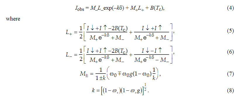
I↓ is the downward radiance (assumed isotropic) incident on the top of the cloud layer, I↑ the upward radiance at the base of the layer, and g the asymmetry parameter. Tc is a representative temperature of the cloud layer.
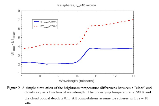
A challenge in cloud masking is detecting thin clouds. Assuming a thin cloud layer, the effective transmittance (ratio of the radiance exiting the layer to that incident on the base) is derived from equation (4) by expanding the exponential. The effective transmittance is a function of the ratio of I↓/I↑ and B(Tc)/I↑. Using atmospheric window regions for cloud detection minimizes the I↓/I↑ term and maximizes the B(Tc)/I↑ term. Figure 2 is a simulation of differences in brightness temperature between clear and cloudy sky conditions using the simplified set of equations (4)-(8). In these simulations, there is no atmosphere, the surface is emitting at a blackbody temperature of 290 K, and cloud particles are ice spheres with a gamma size distribution assuming an effective radius of 10 μm, and the cloud optical depth δ = 0.1. Two cloud temperatures are simulated (210 K and 250 K). Brightness temperature differences between the clear and cloudy sky are caused by non-linearity of the Planck function and spectral variation in the single scattering properties of the cloud. This figure does not include the absorption and emission of atmospheric gases, which would also contribute to brightness temperature differences. Observations of brightness temperature differences at two or more wavelengths can help separate the atmospheric signal from the cloud effect.
The infrared threshold technique is sensitive to thin clouds given the appropriate characterization of surface emissivity and temperature. For example, with a surface at 300 K and a cloud at 220 K, a cloud with an emissivity of 0.01 affects the top-of-atmosphere brightness temperature by 0.5 K. Since the expected noise equivalent temperature of MODIS infrared window channel 31 is 0.05 K, the cloud detecting potential of MODIS is obviously very good. The presence of a cloud modifies the spectral structure of the radiance of a clear-sky scene depending on cloud microphysical properties (e.g., particle size distribution and shape). This spectral signature, as demonstrated in Figure 2, is the physical basis behind the brightness temperature difference tests.
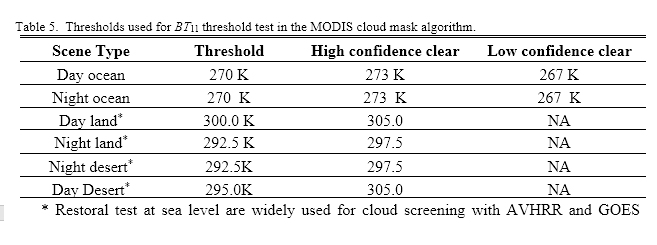
BT11 THRESHOLD (“FREEZING”) TEST (BIT 13)
Several infrared window threshold and temperature difference techniques have been developed. These algorithms are most effective for cold clouds over water and must be used with caution in other situations. Over (liquid) water when the brightness temperature in the 11 μm (BT11) channel (band 31) is less than 270 K, we assume the pixel to fail the clear-sky condition. The three thresholds over ocean are 267, 270, and 273 K, for low, middle, and high confidence of clear sky thresholds, respectively. Note that “high confidence clear” in this case means that BTs warmer than 273 K cannot indicate cloud according to this test. Obviously, clouds may exist at warmer temperatures and may be detected by other cloud tests. See Section 3.2 for a full description of the thresholding and confidence-setting process.
Cloud masking over land surface from thermal infrared bands is more difficult than over ocean due to potentially larger variations in surface emittance. Nonetheless, simple thresholds are useful over certain land features. Over land, the BT11 is used as a clear-sky restoral test. If the initial determination for a pixel is cloudy, that pixel may be “restored” to clear if the observed BT11 exceeds a threshold defined as a function of elevation and ecosystem. Table 5 lists the “freezing test” and clear sky restoral test thresholds. Unless otherwise indicated, all thresholds listed in this document apply to the Aqua instrument. Though most thresholds are identical between Aqua and Terra, there are some small differences due to variations in instrument age and other characteristics.
BT11 - BT12 AND BT8.6 - BT11 TEST (BITS 18 AND 24)
As a result of the relative spectral uniformity of surface emittance in the IR, spectral tests within various atmospheric windows (such as MODIS bands 29, 31, 32 at 8.6, 11, and 12 μm, respectively) can be used to detect the presence of cloud. Differences between BT11 and BT12 is often referred to as the split window technique. Saunders and Kriebel (1988) used BT11 - BT12 differences to detect cirrus clouds—brightness temperature differences are larger over thin clouds than over clear or overcast conditions. Cloud thresholds were set as a function of satellite zenith angle and the BT11 brightness temperature. Inoue (1987) also used BT11 - BT12 versus
BT11 to separate clear from cloudy conditions.
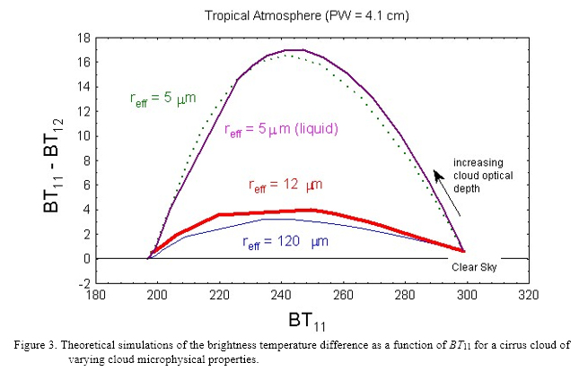
In difference techniques, the measured radiances at two wavelengths are converted to brightness temperatures and subtracted. Because of the wavelength dependence of optical thickness and the non-linear nature of the Planck function (Bλ), the two brightness temperatures are often different. Figure 3 is an example of a theoretical simulation of the brightness temperature difference between 11 and 12 μm versus the brightness temperature at 11 μm, assuming a standard tropical atmosphere. The difference is a function of cloud optical thickness, the cloud temperature, and the cloud particle size distribution.
The basis of the split window and 8.6-11 μm BTD for cloud detection lies in the differential water vapor absorption that exists between different window channel (8.6 and 11 μm and 11 and 12 μm) bands. These spectral regions are considered to be part of the atmospheric window where absorption is relatively weak. Most of the absorption lines are a result of water vapor molecules, with a minimum occurring around 11 μm.
In the MODIS cloud mask, we follow Saunders and Kriebel (1988) in the use of 11-12 μm BTDs to detect transmissive cirrus cloud, with small corrections to the thresholds for nighttime
For more detailed and complete information, view the Cloud Mask Algorithm Theoretical Basis Document (ATBD) near the bottom of the "ATBDs, Plans, and Guides" page at https://atmosphere-imager.gsfc.nasa.gov/documentation/atbds-plans-guides